
Roughly 65% of prototype asset trackers fail early field testing because passive component parasitic capacitance pulls the 32.768 kHz RTC crystal off frequency, preventing the MCU from entering deep sleep. Executing a successful Custom PCB Design for Tracking Devices requires bridging strict RF layout constraints with microampere-level power gating. Standard dev boards won’t cut it. They waste up to 80% of your power budget through active regulators and poor ground plane design.
This guide gives you the precise engineering parameters required to take a tracker from initial schematic to production-ready hardware. You will work through coplanar waveguide routing, antenna matching networks, low-dropout regulator selection, and power-gating topologies that drop sleep currents below 5 µA.
Doing this right takes serious effort. Expect to spend hours tuning matching components on a vector network analyzer, scrubbing your layer stackup for EMI, and debugging board-level leakage paths. But once your design lands, your hardware will survive real-world deployments intact.
Why Is Custom PCB Design for Tracking Devices Necessary Over Off-the-Shelf Modules?
Off-the-shelf modules waste 70% of board space on unneeded interfaces. Purpose-built hardware enables rigid-flex contours, high-density interconnect (HDI) routing, and component-level power gating, dropping sleep current to microamps.
Engineered Hardware vs. Off-the-Shelf Breakouts
| Metric | Off-the-Shelf Board | Custom Tracking PCB |
|---|---|---|
| Sleep Current | 1.5 mA to 5 mA | 3 µA to 12 µA |
| Board Thickness | 1.6 mm rigid | 0.4 mm rigid-flex |
| Component Density | Low (0603 passive min) | High (0201/01005 HDI) |
Breakouts suit early firmware testing. They fail in rugged enclosures. Unnecessary USB transceivers and linear regulators waste energy. A 2.5 mA idle draw kills a 500 mAh battery in 8 days. Dropping sleep draw to 4 µA extends field life past 3 years.
Fitting a cellular modem, GNSS receiver, nano-SIM slot, and 9-axis MEMS accelerometer into tight housings requires blind vias and 0201 passives. Shifting trace clearances near battery clips by 0.15 mm creates EMI coupling.
Relying on custom PCB design services provides the HDI layer stackups, low-noise RF traces, and power-gating topologies required for field reliability. You avoid costly revs and keep BOM targets intact.
- Eliminate parasitic drain from power LEDs and onboard UART chips.
- Flex thin circuit layers around lithium polymer batteries to maximize space.
How Do You Choose Between GNSS, Cellular, and BLE Architectures for Location Tracking?
Architectural Trade-offs and Decision Criteria
GNSS active acquisition draws 20 mA to 40 mA with a 30 seconds cold start. Cellular triangulation offers 100 meters accuracy at under 15 µA sleep current.
When designing a pet tracking PCB, update schedules under two minutes require rechargeable lithium chemistry for your board.
| Architecture | Active Current | Operational Range | Location Accuracy |
|---|---|---|---|
| Multi-Constellation GNSS | 25 mA – 45 mA | Global Outdoor Direct Line-of-Sight | 1.5 m – 5 m |
| LTE-M / NB-IoT | 100 mA – 250 mA Tx Peak | Global Cellular Network Range | 100 m – 1000 m |
| Bluetooth Low Energy (BLE 5.x) | 4 mA – 8 mA | Local Proximity (Under 100 m) | 1 m – 3 m (RSSI / AoA) |
What Is the Ideal Layer Stackup and Antenna Matching Design for GPS Trackers?
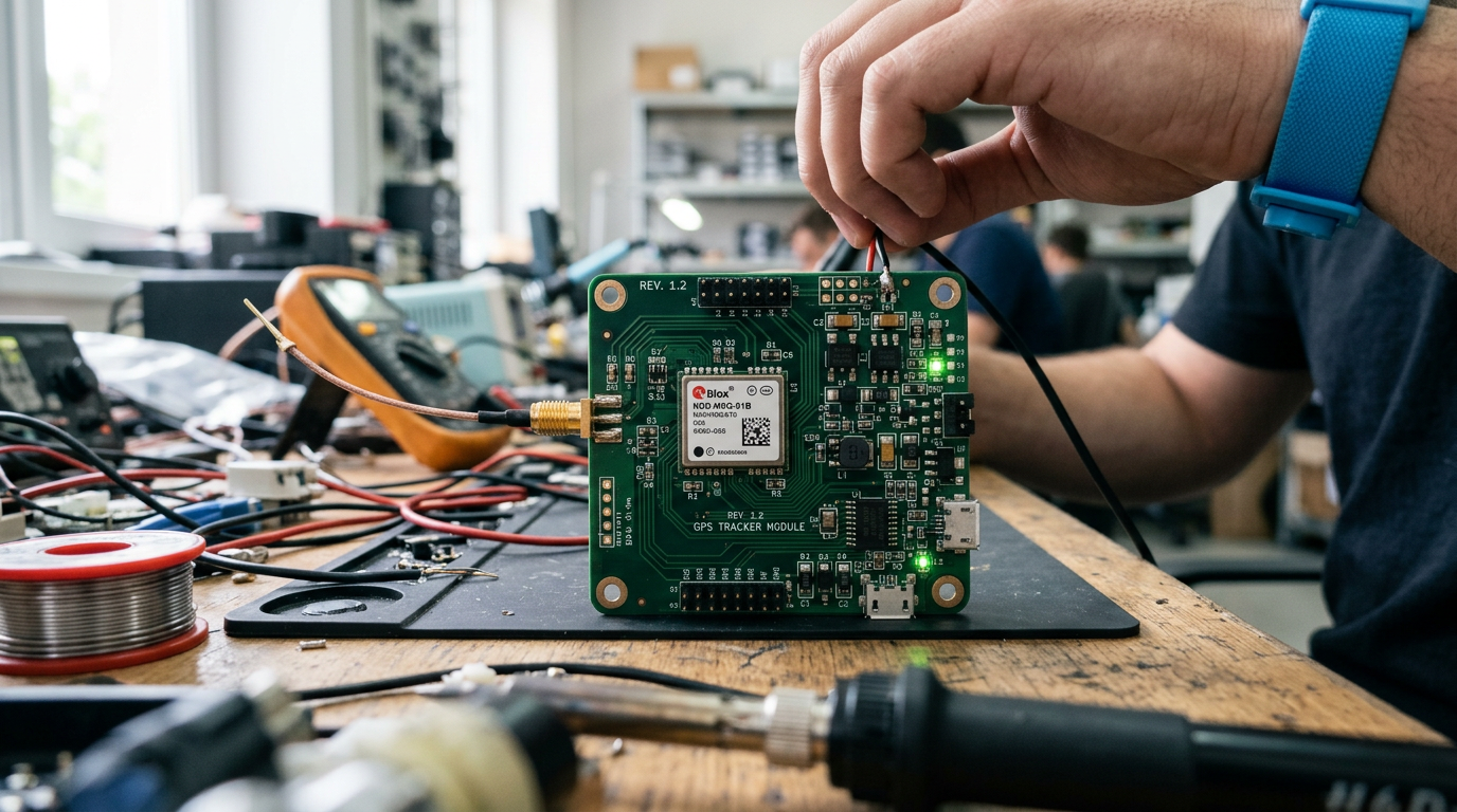
The ideal layer stackup for a GPS tracker uses a 4-layer configuration: Top Signal, Inner Ground, Inner Power, and Bottom Signal. Layer 2 serves as a continuous ground plane directly beneath the 1.575 GHz RF microstrip, maintaining a strict 50-ohm characteristic impedance and securing a VSWR below 1.5 with a Pi-matching network.
Stackup Setup and Noise Isolation
When executing custom PCB design for tracking devices, stackup spacing dictates your RF integrity. Place your RF feedline on Layer 1 over an uninterrupted Layer 2 ground plane. In early builds, digital switching noise from a 2.1 MHz DC-DC buck regulator coupled directly into the Low-Noise Amplifier (LNA) supply trace. That ripple degraded carrier-to-noise density (C/N0) by 12 dB-Hz. Solve this by isolating the LNA power rail using a dedicated ferrite bead with 600-ohm impedance at 100 MHz alongside 10 pF and 100 nF decoupling capacitors placed within 2 mm of the LNA pin.
Antenna Pi-Matching and VNA Calibration
Proper antenna tuning determines the function and design of GPS PCBs. Calibrate your Vector Network Analyzer (VNA) using a standard 1-port SOLT procedure across a 1.50 GHz to 1.65 GHz sweep. In your CAD software—such as KiCad or Altium—calculate a 0.50 mm microstrip width over a 0.20 mm FR4 dielectric layer (εr = 4.5) to achieve 50-ohm impedance. Tune the Pi-matching network using a 5.6 nH series inductor paired with 1.2 pF and 0.8 pF shunt capacitors. This specific combination drops S11 reflection down to -16.5 dB, guaranteeing maximum energy transfer at 1.57542 GHz.
Why Do Most Tracking PCB Prototypes Fail in Field Deployment?
Most tracking PCB prototypes fail in the field because lab bench conditions mask physical realities like casing detuning, un-gated power leaks, and thermal trapping inside sealed enclosures. Open-source designs rarely account for the dielectric constant of an IP67 housing, which instantly shifts antenna resonant frequencies and drops carrier signal strength below usable margins.
When executing Custom PCB Design for Tracking Devices, standard layouts break down under real-world stress due to three main causes:
- Antenna detuning from plastic housing: Placing a 1575.42 MHz ceramic GPS patch antenna inside a 3mm polycarbonate enclosure shifts its center frequency down by 15–30 MHz through dielectric loading. Without tuning via a vector network analyzer inside the final casing, lock times multiply and signal attenuation spikes.
- Un-gated sleep leakage: A 10 kΩ pull-up resistor on an I2C sensor bus tied to an un-gated rail drains 330 µA continuously in deep sleep. That tiny leak destroys a multi-year coin cell power budget in six weeks.
- Thermal trapping in IP67 seals: LTE modules draw 2A peak pulses during transmission. In an unventilated IP67 enclosure, rapid uplink cycles drive internal ambient temperatures past 85°C, triggering thermal regulator shutdowns and clock oscillator drift.
Community schematic templates skip high-side load switch isolation and localized copper thermal relief planes. Relying on these reference designs for your first location tracker PCB build works fine on a bench. But long-term reliability demands re-tuning RF paths inside the final enclosure shell and aggressively power gating every peripheral rail.
How Do You Implement Low-Power Firmware States and Power Gating Circuitry?
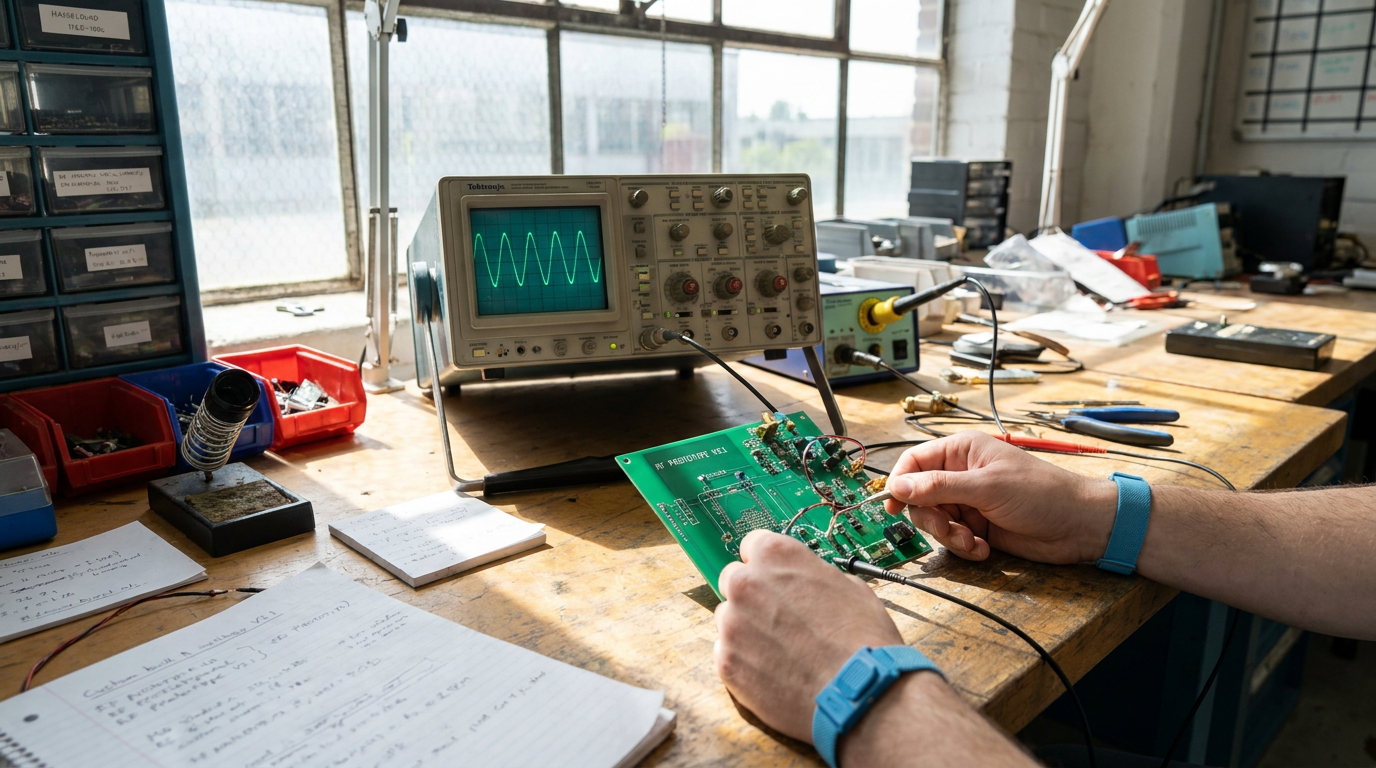
Implementing low-power firmware states and power gating requires isolating peripheral ICs using P-channel MOSFET load switches controlled by MCU GPIOs, cutting quiescent leakage. Pair hardware cutoffs with low-power firmware sleep modes triggered by RTC interrupts or accelerometer motion thresholds, driving active tracking power down from a 45mA active tracking state to a 3.8µA deep sleep state.
Hardware Power Gating Setup
GNSS receiver modules drain batteries rapidly if left powered in standby mode. Connect a high-side P-channel MOSFET between the system power rail and the GNSS VCC pin. Pull the gate high with a 100kΩ resistor to keep the switch off by default. Drive the gate low through an MCU GPIO pin or N-channel driver to energize the module only during satellite acquisition. This setup drops power draw from a 45mA active tracking state to 3.8µA deep sleep, preventing parasitic leakage through RX/TX lines by setting those GPIO pins to analog high-impedance before gating off power.
Firmware Interrupts and Fabrication Rules
Configure your microcontroller to enter deep sleep immediately after publishing coordinates. Set an onboard RTC to fire an external wake-up interrupt every four hours for stationary check-ins. For motion-based tracking, configure an ultra-low-power accelerometer to trigger a hardware interrupt when movement crosses a 35mg threshold for longer than 20ms. When routing dense interconnects for Custom PCB Design for Tracking Devices, refer to a wearable PCB online fabrication guide. Standard automated board houses require strict 4-mil trace/space tolerances, 0.8mm board thickness, and high-density interconnect rules to prevent solder bridging between tiny 0402 components and load-switch packages.
What Is the 3W Rule for PCB Design and How Does It Prevent RF Interference?
The 3W rule states that the center-to-center distance between two adjacent microstrip traces must equal at least three times the trace width. This physical separation lowers capacitive crosstalk and mutual inductive coupling by roughly 70%, protecting sensitive traces in dense board layouts.
In a compact layout for custom PCB design for tracking devices, fast digital edges cause severe RF performance loss. A 24 MHz SPI clock bus driving an onboard IMU creates sharp square waves rich in high-order harmonics. If routed parallel to a 1575.42 MHz GPS receiver feedline without proper spacing, magnetic and capacitive coupling injects broadband noise into the low-noise amplifier, degrading carrier-to-noise ratio (C/N0) by 3 dB to 6 dB.
When to Implement 10W Spacing and Guard Vias
High-power cellular trackers transmitting at +23 dBm demand aggressive signal isolation. A standard 3W gap cannot suppress high-frequency power amplifier harmonics or DC-DC buck converter switching spikes.
- 10W Rule: Separate RF traces from aggressive switching nodes by ten trace widths center-to-center, suppressing electromagnetic coupling by over 98% and reducing crosstalk to under -40 dB.
- Guard Via Fences: Place grounded vias along coplanar waveguides at a pitch under lambda/10 (roughly 1.8 mm for GPS L1) to tie top ground floods to the internal plane when layout gaps fall below 3W.
As documented in almost every practical forum guide for GPS tracking PCBs, spatial separation rules offer zero protection if you split the reference plane. Routing traces over ground cutouts forces return currents to loop, creating efficient loop antennas that completely undermine your 3W isolation.
Can ChatGPT Do PCB Design or Generate Reliable Gerber Files?
ChatGPT cannot generate reliable Gerber files or directly design physical PCB layouts. While AI models excel at writing basic scripting plugins or organizing bill-of-materials data, they cannot perform spatial routing, calculate 50-ohm RF trace impedance, or model parasitic capacitance and thermal dissipation across solid copper planes.
Where Generative AI Fails in EDA Workflows
Generative AI frequently hallucinates IC pinouts and lacks 3D spatial awareness. In custom PCB design for tracking devices, an inaccurate trace width calculation or missing return path will degrade your GNSS receiver sensitivity by 10 dB or corrupt cellular transmission under 4G burst loads. LLMs do not run finite element method (FEM) solvers. They cannot predict how a 4-layer 1.6mm FR-4 stackup affects differential pair skew, nor can they handle thermal plane relief near power-gating MOSFETs drawing peak currents over 2A. Text-based AI cannot output valid Gerber RS-274X coordinate geometry without introducing syntax corruption that fails factory CAM checks.
Safe Automation vs. Human Sign-Off
Treat AI as a helper for low-risk administrative tasks. Let it write Python scripts for KiCad to automate silkscreen alignment, format netlists, or parse datasheet tables. Leave physical schematic capture, stackup rules, and Gerber export to dedicated EDA software verified by human sign-off. For university students exploring viva safe hardware project ideas, using AI to draft board automation scripts while personally routing the antenna matching network demonstrates true engineering discipline without risking non-functional hardware during your final bring-up.
How Do You Route High-Frequency RF Traces and Antenna Feedlines?
Route 1.575 GHz GPS and 2.4 GHz BLE traces using grounded coplanar waveguide (GCPW) geometry to maintain 50-ohm impedance over an unbroken Layer 2 ground plane. Apply 3W copper pour clearance and 45-degree mitered bends. Space feedline ground vias at λ/10 intervals—roughly 6 mm for 2.4 GHz on FR-4.
Altium’s high-speed design guidelines emphasize precise stackup impedance control alongside automated end to end tracking of PCB design constraints. To pass FCC Part 15 or CE RED testing, enclose GNSS front-ends in a soldered metal shielding can secured by ground vias spaced 2 mm to 3 mm apart.
How Much Does It Cost to Have a Custom PCB Design Built and Assembled?
Building a custom tracking device PCB costs between $1,000 and $5,000 for low-volume prototypes, while high-volume production drops unit prices under $15. Initial Non-Recurring Engineering (NRE) design fees account for $500 to $3,000 of that initial budget, while bare board fabrication and assembly stencil setup fees make up the remainder.
Breakdown of Prototyping vs. Volume Costs
When executing custom PCB design for tracking devices, your total expense divides between fixed engineering overhead and variable production charges. Engineering providers offering turnkey electronic design services charge NRE fees to convert your architecture block diagram into finished Gerber, ODB++, or IPC-2581 manufacturing files.
Typical prototype expenses split into three distinct categories:
- Schematic & Layout Engineering: $500 to $3,000 depending on multi-constellation RF complexity.
- Bare Board Fabrication: $20 to $100 for an initial batch of 5 to 10 prototype boards.
- SMT Stencil & Setup: $15 to $50 for laser-cut stainless steel stencils and automated feeder setup.
Optimizing Unit Economics at Scale
Single prototype units cost between $100 and $250 per assembled board due to SMT line configuration overhead. Scaling past 1,000 units brings component reel discounts and automated throughput into play, reducing per-unit assembly costs down to $12–$25.
You keep expenses under control by choosing standard 0402 passive components instead of 0201 packages. Standard 0402 passives lower pick-and-place defect rates. Furthermore, sticking to low-cost 4-layer stackups (such as 1.6mm FR-4 with 1oz copper) avoids custom lamination surcharges. Avoid blind or buried vias unless high-density micro-BGA packages leave you no choice.
How Do I Build My Own GPS Tracker from Schematic to Enclosure?
Building a custom GPS tracker requires selecting an integrated MCU and GNSS module, capturing the schematic in software like KiCad, laying out RF trace paths with 50-ohm impedance control, and fitting the assembled board into an IP67 enclosure after validating power draw and cold-start lock times on the bench.
From Schematic to Hardware Deployment
Executing a custom PCB design for tracking devices requires a disciplined, step-by-step workflow from part selection to physical housing:
- Component Selection: Pair an ESP32-C3 microcontroller with a u-blox MAX-M10S GNSS module, an MCP73831 battery charger circuit, and a 3.7V LiPo cell driven by an ultra-low quiescent LDO like the AP7361C.
- Schematic & PCB Layout: Draft your schematic in KiCad or EasyEDA. Set DRC constraints to 0.15mm clearance and 0.2mm trace width. Route a 50-ohm coplanar waveguide feedline directly to your passive ceramic patch antenna.
- Ground Planes: Flood top and bottom layers with copper ground plane pours, placing a dense array of via fences around the RF trace to isolate RF energy from switching noise.
- Benchtop Validation: Profile power draw using a benchtop multimeter to confirm sleep states under 15µA. Verify outdoor cold-start TTFF (Time-To-First-Fix) hits 26 seconds, dropping to 1 second during warm starts.
- 3D Enclosure Fit Check: Export your populated board as a 3D STEP file into Fusion 360 to verify mechanical clearance for battery connectors, antenna orientation, and mounting bosses before 3D printing.
This end-to-end engineering pipeline offers strong practical value when executing fyp ideas for engineering students who need to deliver reliable, field-ready physical hardware.
Which Online PCB Fabrication Services Offer Fast Prototyping and SMT Assembly?
Fast prototyping and SMT assembly for custom PCB design for tracking devices rely on vendors like JLCPCB, PCBWay, and ALLPCB. JLCPCB excels at fast turnaround on standard FR4 layers, while PCBWay leads in RF substrates like Rogers 4350B, and ALLPCB offers automated turnarounds for high-speed production runs.
| Platform | SMT Turnaround | In-Stock Components | RF Substrate Support |
|---|---|---|---|
| JLCPCB | 24–48 hours | 500,000+ parts | Standard FR4 SMT |
| PCBWay | 3–5 days | Custom global sourcing | Rogers 4350B stackups |
| ALLPCB | 48–72 hours | Essential passives | Special order laminates |
Substrate Selection and Turnkey Scaling
Standard FR4 works well for basic power distribution and slow digital logic. However, 1.575 GHz GNSS receivers and 2.4 GHz Wi-Fi antenna feedlines require predictable dielectric constants. PCBWay easily supports hybrid stackups using Rogers 4350B over FR4 inner cores, keeping RF attenuation below 0.1 dB/cm. JLCPCB limits low-cost automated SMT to standard FR4 laminates, which causes higher RF signal loss on compact tracker layouts. Short traces mitigate this, but tight designs suffer. ALLPCB sits in the middle, offering fast turnaround for standard substrates while charging premium expediting fees for custom RF stacks.
When analyzing a robotics hardware integration case study, rapid turnkey prototyping demands balancing off-the-shelf part libraries against long component lead times. Moving from five prototype boards into full turnkey box-build production shifts your engineering focus. You must verify component sourcing channels, validate panelization tooling, demand X-ray inspection for fine-pitch BGAs, and confirm that enclosure fitments pass vibration testing. Skipping these steps risks costly line re-tooling.
Before you route your first trace in your EDA tool, measure the sleep current draw of your MCU and cellular modem on a breakout board using a dedicated current profiler. You want to see your sleep baseline flatline below 15 µA without floating GPIO pins causing leakage spikes. That stable microamp line is your signal that your power gating schematic actually works before you order physical copper.
A custom board will not fix flawed system architecture or broken power math. If your design demands a 1-second GNSS update rate on a 200 mAh battery, custom routing cannot beat physical power limits. Do not bother building custom hardware if your enclosure fits standard development kits and off-the-shelf modules meet your thermal spec. Custom layouts exist for tight physical constraints, custom antenna matching, and strict millimeter-level spatial constraints. Validate your sleep currents on the bench first, lock down your schematic, and only then start your stackup layout.
Frequently Asked Questions
How much does it cost to have a custom PCB design?
Custom PCB design costs range from a few hundred dollars for simple two-layer boards to over $10,000 for complex multi-layer tracking devices with RF integration. Total pricing depends on schematic complexity, layer count, component availability, and required certifications like FCC or CE. You can optimize costs by selecting standard component footprints and reducing board stack-up layers during early prototyping.
Can ChatGPT do PCB design?
ChatGPT cannot directly generate physical PCB layout files, but it can assist you by writing code scripts, recommending schematics, and drafting design specifications. While it helps brainstorm component selection or write Python scripts for CAD tools like KiCad, you still need dedicated EDA software to route traces and handle signal integrity. You must manually verify all AI-generated pinouts and netlists before fabrication.
What is the 3w rule for PCB design?
The 3W rule states that the distance between adjacent microstrip traces must be at least three times the width of a single trace to minimize crosstalk. Measuring center-to-center, this spacing reduces electromagnetic coupling between parallel lines by roughly 70 percent. You should apply this guideline to high-speed clock signals and sensitive RF traces in your tracking device layout to maintain clear signal integrity.
How do I build my own GPS tracker?
Building your own GPS tracker requires combining a microcontroller, a GNSS module, a cellular or LoRa transceiver, and a power management circuit onto a unified PCB. You begin by selecting low-power components, drafting the schematic, and routing the PCB with proper antenna impedance matching. Once fabricated, you solder the parts and program your firmware to parse NMEA location data and transmit it to your cloud platform.
What is the difference between active and passive patch antennas on tracking PCBs?
Active patch antennas include an integrated Low Noise Amplifier (LNA) requiring power, whereas passive patch antennas consist solely of the radiating element without built-in signal amplification. You should choose an active antenna if your tracking device has long cable runs or operates in weak satellite signal environments. However, passive antennas save precious battery life and circuit space, making them ideal for ultra-compact, low-power IoT designs.
References and Technical Standards
A practical robotics hardware integration case study reveals the stark gap between a clean CAD drawing and an operational cell. You can write clean controller logic, but an unshielded Variable Frequency Drive cable will still corrupt your encoder signal over CAN bus if routed together through the same wire tray.
This guide provides the physical layout rules, functional safety setups, ROS 2 bus configurations, and edge AI execution pipelines needed to marry hardware with code. It gives you the complete engineering framework to build a functional autonomous system, whether you are deploying an industrial cell or finishing a Final Year Project.
Success requires serious sweat equity. You must audit ground loops, calculate power drops across 24-volt rails, and tune actuator timing until packet jitter disappears. There are no shortcuts here—just direct, practical execution.
Architecting the Perception-to-Action Loop in Industrial Workcells
The perception-to-action loop dictates how fast your workcell reacts to its physical environment. Sensors capture raw data—like point clouds or RGB-D frames—and stream it to an inference engine. The model calculates spatial targets, sending Cartesian coordinates to a motion trajectory generator. Inverse kinematics algorithms then convert those spatial paths into joint motor torque commands. Mathematically, loop delay equals sensor exposure time plus frame transport, model inference duration, trajectory calculation, and bus latency: Ttotal = tsensor + ttransport + tinfer + tplan + tbus. If total latency exceeds your physical control cycle window—typically 1 to 4 milliseconds for high-speed pick-and-place—your robot arm drifts off its path. In physical AI integration workflows, minimizing each variable keeps payloads from overshooting targets or dropping items.
Centralized Compute vs. Edge Topology
Choosing where to calculate trajectories shapes system architecture. Centralized systems feed raw sensor data directly to a single industrial PC over high-bandwidth links. The central computer handles vision processing, spatial planning, and safety logic on one memory bus. Distributed edge topologies offload feature extraction to smart cameras or specialized accelerators, passing lightweight spatial coordinates down to dedicated controllers. Centralized builds lower physical component counts, but heavy camera streams can saturate system buses. Edge topologies decouple heavy vision compute from motion loops, keeping motor timing deterministic.
| Topology Type | Trajectory Latency | Bandwidth Load | Fault Isolation |
|---|---|---|---|
| Centralized Industrial PC | < 2 ms (Shared RAM) | High (Raw point clouds) | Single point of failure |
| Distributed Edge Nodes | 5 – 15 ms (Network hop) | Low (Pre-processed poses) | Isolated to local node |
| Hybrid (Edge Vision + IPC) | 2 – 4 ms (Synchronized) | Medium (Vector streams) | Segmented fault domains |
Serial Bus Constraints vs. Industrial Ethernet
Hardware communication lines frequently bottleneck loop throughput. Legacy serial interfaces like RS-485 or standard CAN bus struggle with multi-axis state updates. A standard CAN frame carries 8 bytes of payload at 1 Mbps maximum speed. Transmitting six joint angles and motor drive telemetry saturates the bus capacity, raising execution jitter above 10 milliseconds. That is too slow for dynamic obstacle avoidance.
Industrial Ethernet protocols—such as EtherCAT and PROFINET IRT—eliminate this latency bottleneck using hardware-level synchronization. EtherCAT processes frame data on the fly using dedicated chips inside slave drives. A single master frame passes through every node in the workcell, updating target positions and reading actual drive encoders in a sub-millisecond sweep. If your system requires real-time path updates, selecting EtherCAT over legacy fieldbuses drops trajectory tracking errors. Building a reliable system means balancing these physical hardware trade-offs, a core principle detailed in any practical industrial robotics automation guide. When evaluating your next robotics hardware integration case study, verify that protocol clock synchronization jitter stays below 1 microsecond.
Step-by-Step Robotics Hardware Integration Case Study Walkthrough
Bench Testing and Mechanical Setup
Executing a 6-axis articulated arm deployment demands absolute control during initial staging. In this robotics hardware integration case study, the project followed a strict 12-week deployment timeline. Weeks one through four focused entirely on bench isolation. Mount your master controller onto DIN rails and establish a unified ground plane before connecting power. Power the logic board via an isolated 24V DC desktop supply during this phase. You must validate electrical communication and logic routing before bolting an arm to the factory floor. Skipping bench isolation will cost you time when troubleshooting physical faults later.
Start by mapping your control bus hardware. For serial telemetry between the primary controller and the gripper end-effector, wire an RS-485 transceiver using a standard half-duplex topology:
- Connect Pin 1 (RO) to Controller UART RX, Pin 4 (DI) to Controller UART TX, and short Pins 2 and 3 (RE/DE) to a single dedicated GPIO pin for direction switching.
- Route differential lines A and B over shielded twisted-pair cabling with a 120-ohm termination resistor placed across A and B at each physical end of the bus.
Before sending motion commands, configure conservative safety ceilings inside your motor drive software interface. Set joint 1 and joint 2 maximum torque limits to 35.0 Nm. Limit joint 3 to 14.5 Nm, and cap joints 4 through 6 at 8.2 Nm. These software caps prevent mechanical strain or gear shearing if your kinematics solver outputs an unmapped vector during initial trajectory tuning.
Bus Diagnostics and Torque Calibration
Log exact register values from your drive controller interface during bench tests. Misconfigured timing parameters cause silent frame loss before you ever move a joint.
| Joint / Node Axis | Baud Rate | Torque Ceiling | Target Polling Interval |
|---|---|---|---|
| Joint 1 & 2 (Base/Shoulder) | 115,200 bps | 35.0 Nm | 2.0 ms |
| Joint 3 (Elbow) | 115,200 bps | 14.5 Nm | 2.0 ms |
| Joints 4–6 (Wrist Axes) | 115,200 bps | 8.2 Nm | 1.0 ms |
| End-Effector Tool Node | 57,600 bps | 4.5 Nm | 5.0 ms |
Field Deployment and Noise Mitigation
Transitioning the assembly from the bench to the production cell in week six brought immediate hardware failures. During the first full-speed physical run, energizing the adjacent 480V three-phase conveyor motor corrupted low-voltage communication lines. Joint 2 and Joint 4 optical encoders dropped packets every 400 milliseconds. The serial transceiver logged continuous CRC frame errors on the diagnostic terminal. The oscilloscope confirmed 18-volt voltage spikes riding on the logic line. High-voltage inductive spikes from motor contactors coupled directly into the unshielded 24V DC logic rail.
Raw noise wiped out data frames. You cannot fix bad hardware physics with software patches. Power-line filtering resolved the signal corruption. First, install a dual-stage differential-mode LC low-pass filter on the primary 24V DC bus powering the logic boards. Next, clamp high-permeability snap-on ferrite beads onto both ends of the encoder cables. Finally, anchor cable shielding to the main backplate using 360-degree EMI grounding clamps.
Troubleshooting UART Buffer Overruns
During extended physical runs, you might see packet drops even after fixing electrical interference. If your main microcontroller handles forward kinematics calculations and serial polling on a single thread, high CPU utilization delays the RS-485 read cycle. Setting the UART receiver FIFO threshold to 8 bytes instead of 1 byte fixes buffer overflows. Assign the serial polling routine to a hardware interrupt driven by a dedicated hardware timer operating at 500 Hz. Store incoming telemetry bytes in a 256-byte ring buffer so incoming data frames do not wait on kinematic math execution.
Once power-line filtering was applied, signal corruption vanished entirely. Data packet loss dropped to zero on the scope. The 6-axis arm completed continuous payload cycles across its 1.2-meter reach envelope without dropping safety locks. Comprehensive hardware and software integration services account for these noisy industrial environments long before final sign-off. By week twelve, the cell passed full operational validation, maintaining a repeatable 18.5-second pick-and-place cycle without a single bus reset.

Bridging Edge AI Models to Actuators and Manipulators
From Spatial Tensors to Motor Drives
When an edge AI model processes a camera frame, it outputs a bounding box or pose estimation tensor. That tensor lives in spatial coordinates. Your motor drives do not care about spatial coordinates. They only understand pulses, duty cycles, and fieldbus packets.
To bridge this gap, raw tensor outputs pass through inverse kinematics (IK) algorithms to calculate specific joint angles. A low-level trajectory planner converts these target angles into smooth time-series steps. For stepper motor drives, the controller translates step counts into pulse-and-direction signals. Pulse frequency dictates velocity, while total pulse counts establish final position. For brushless DC (BLDC) drives, target coordinates convert into pulse-width modulation (PWM) commands or CANopen fieldbus position frames. The drive modulates three-phase current across stator windings to produce torque.
Acceleration Capping and Mechanical Protection
Neural networks generate trajectories optimized for visual loss functions, not mechanical longevity. An inference engine might output a spatial coordinate jump between consecutive frames due to optical occlusion or sensor noise. Feeding raw inference points directly to hardware creates immediate mechanical failure risks.
In practice, a deterministic velocity-jerk filter sits between your inference output and the drive controller. If an AI trajectory requests 400 rad/s² of joint acceleration, but your harmonic drive maximum rating is 120 rad/s², the filter clips the step. The safety loop overrides the raw neural network command. This prevents mechanical binding, high current spikes, and chipped gear teeth while maintaining the intended vector direction. Analyzing how these software overrides prevent hardware lockup is a core component of any complete robotics hardware integration case study.
Selecting BLDC vs. Open-Loop Stepper Actuators
Choosing your motor architecture dictates how model predictions translate into physical work cell action. Open-loop steppers count pulses and assume physical compliance. Closed-loop BLDC motors rely on encoder feedback to ensure target positions match commanded coordinates under dynamic loads.
| Metric | Open-Loop Stepper Motor | Closed-Loop BLDC Motor |
|---|---|---|
| Position Verification | None (assumes zero step loss) | Continuous via absolute/incremental encoder |
| Torque at High RPM | Drops off sharply above base speed | Sustained across rated velocity profile |
| Thermal Behavior | Draws full current at idle | Current scales dynamically with actual load |
| Response to Obstructions | Stalls and loses absolute position reference | Triggers soft-torque limits or safety faults |
Select open-loop steppers when payload masses stay constant, motion speeds remain under 300 RPM, and system costs must remain minimal. Select closed-loop BLDC drives for dynamic payloads, high-speed pick-and-place routines, or force-sensitive manipulation. When delivering AI machine learning deployment services, real-time current and position feedback from BLDC encoders allows edge models to detect physical contact events directly, closing the control loop at the hardware seam.
Benchmarking Industrial Automation Performance Metrics
Measuring hardware performance requires moving past raw mechanical speed. You need hard numbers on system responsiveness, physical reliability, and deterministic software execution. When you evaluate a robotics hardware integration case study, the primary metrics center on Overall Equipment Effectiveness (OEE), end-to-end cycle time, control system jitter, and bus communication latency. Legacy standalone machines often operate in isolated hardware silos. That disconnect causes severe communication bottlenecks between programmable logic controllers (PLCs) and peripheral sensors. Modern integrated architectures bypass these transport delays by processing sensor feeds directly near the motor drive interface. You get faster reaction times, predictable joint trajectories, and lower mechanical wear.
Core Operational Metrics for Integrated Workcells
To benchmark your workcell accurately, you must isolate mechanical motion delays from software execution lag. Track these key performance indicators during initial hardware commissioning:
- Deterministic Latency: The exact time elapsed between initial sensor signal acquisition, control loop calculation, and the resulting motor torque command execution.
- Overall Equipment Effectiveness (OEE): A composite measurement evaluating operational availability, performance rate, and overall output quality yield.
- Mean Time Between Failures (MTBF): The continuous operational run time hardware components achieve before requiring physical maintenance.
- Cycle Time Variation: The standard deviation in task completion times when the system operates under fluctuating payload conditions.
Legacy industrial setups hit performance ceilings because sensor signals pass through multiple protocol conversion bridges before reaching the primary controller. When you integrate custom edge processing units directly with digital servo drives, interface latency drops. Published robotic automation case studies show that unified hardware-software control loops reduce bus communication jitter down to sub-millisecond windows. That tight timing window directly increases hourly pick-and-place output without forcing mechanical joints past their maximum rated torque limits. It also reduces mechanical chatter, extending gearhead lifespan.
Industry Benchmarks and Market Trends
Global market data from the International Federation of Robotics highlights clear shifts across modern industrial automation facilities. Their analysis of global robot supplier trends documents a steady transition toward decentralized control hardware equipped with real-time fieldbus networking. Traditional standalone machinery cannot maintain the tight feedback loops required for dynamic trajectory modification. By swapping disconnected system components for synchronized communication networks such as EtherCAT or CANopen, you eliminate protocol conversion delays entirely. This architectural shift allows multi-axis manipulators to adjust motion paths mid-stroke based on vision inputs.
Comparing your deployment against published performance standards prevents costly over-engineering during the initial design phase. Never spend your budget on oversized structural frames to compensate for poor positional control software. Instead, prioritize high-resolution feedback encoders, low-latency motor drives, and deterministic fieldbus hardware. A lightweight manipulator using synchronized driver firmware easily outperforms a heavy, rigid arm hindered by legacy serial interfaces and uncalibrated controller gains. Measure sensor-to-actuator delay early in prototyping, test under heavy bus traffic, and base every hardware decision on verifiable operational benchmarks.
Failure Mode: Control Jitter Under Bus Saturation
A common failure during commissioning is control loop starvation. This happens when high-bandwidth sensor payloads—like uncompressed vision streams—share a physical channel with real-time motion commands. The resulting packet collisions spike latency from 250 microseconds up to 12 milliseconds. Your drives lose synchronization, triggering hardware e-stops or severe mechanical chatter. Fix this by isolating heavy payload data onto a dedicated secondary subnet, leaving your real-time fieldbus restricted strictly to cyclic motor commands and safety signals.
Consider a workcell moving a 5 kg load at 2.0 meters per second. A latency jump of 10 milliseconds drifts the physical tool center point by 20 millimeters before the controller reacts. You cannot fix that drift with mechanical tolerances. Deterministic bus timing solves it.
| Control Integration Model | Mean Bus Latency | Cycle Jitter Variance | Failure Risk |
|---|---|---|---|
| Legacy PLC Bridge (Serial) | 20.0 ms | ±8.5 ms | Buffer overflow, positional drift |
| Direct Fieldbus (EtherCAT) | 0.5 ms | ±0.05 ms | Bus saturation under unmanaged traffic |
Selecting Controllers, Sensors, and Bus Protocols
Matching Communication Protocols to Control Loops
Selecting the right bus protocol dictates your system update frequency and deterministic control. When analyzing a robotics hardware integration case study, determinism matters more than raw throughput. If your drive control loop misses its execution window by three milliseconds, high-precision arm movements fail or trigger axis fault trips.
| Protocol | Bandwidth | Jitter | Max Cable Length |
|---|---|---|---|
| EtherCAT | 100 Mbps | < 1 µs | 100 m per segment |
| CANopen | 1 Mbps (at 40m) | 100 µs to 1 ms | 1000 m (at 20 Kbps) |
| PROFINET IRT | 100 Mbps to 1 Gbps | < 1 µs | 100 m per segment |
Use EtherCAT when multi-axis motion synchronization demands sub-microsecond precision across servo drives. EtherCAT frame processing happens in hardware on the slave controller chip, allowing cycle times down to 125 microseconds. CANopen works well for simpler low-speed sensor networks, gripper actuators, or battery management systems where cable runs exceed 100 meters and modest data rates suffice. PROFINET IRT suits factory-wide PLC networks where safety protocols like PROFIsafe share standard Ethernet topology.
Evaluating 3D LiDAR and Stereo Vision
Dynamic indoor environments present lighting shifts, dust, and moving obstacles. Choosing between 3D LiDAR and stereo cameras comes down to surface reflectivity and computational headroom. 3D LiDAR measures distance directly via time-of-flight. It remains unaffected by direct sunlight glare or featureless warehouse walls, delivering consistent geometry for localization algorithms. Solid-state and mechanical 3D LiDAR sensors yield uniform point density regardless of visual contrast, though they add weight and power draw to mobile platforms.
Stereo vision cameras provide dense RGB spatial maps suitable for neural network classification. They cost significantly less than multi-layer LiDAR units. The trade-off is high processing load on your host controller and sensitivity to lighting variations. If your workcell operates in dark spaces or handles mirror-finished metal sheets, stereo depth calculations degrade quickly. Building reliable custom robotics development solutions often requires combining both: LiDAR for primary SLAM and stereo vision for object identification.
Isolating Sensor Lines from Motor Drive Noise
High-voltage pulse-width modulation motor drives generate severe electromagnetic interference (EMI). When an inverter switches at 16 kHz across a 48V or 400V bus, rapid current transitions radiate noise into nearby analog sensor traces. Unshielded 0–10V analog signals pick up voltage spikes, creating phantom sensor readings or tripping controller interrupts.
Stop noise before it reaches your signal processor. Convert raw analog readings to differential digital currents—such as 4–20mA loops or RS-485—right at the sensor interface. Run motor power leads and signal wiring through separate metal conduits, maintaining at least 30 centimeters of separation. Add ferrite chokes near drive terminals to suppress common-mode noise. Ensure your analog-to-digital converters use differential inputs with high common-mode rejection ratios. Always ground cable shields at a single star point inside the control panel to eliminate ground loops that corrupt low-voltage data.

Functional Safety Standards and ISO Compliance Constraints
ISO 13849-1 Performance Level Requirements
Designing a human-robot collaborative workcell requires strict adherence to ISO 13849-1. This standard governs the functional safety of machinery control systems. When human operators share physical space with industrial manipulators, your risk assessment will usually demand Performance Level d (PLd) or Performance Level e (PLe). Achieving PLd requires your system architecture to maintain dual-channel hardware monitoring and a Diagnostic Coverage (DC) of at least 60%. PLe sets a higher bar. It requires Category 4 architecture, where a single component fault will not lead to a loss of the safety function. Software checks alone will not pass inspection. You must mirror every critical safety sensor across independent hardware lines.
Hardwired Emergency Stop Architecture
Physical emergency stop circuits must operate independently of your main application code. Standard IEC 60204-1 specifies functional requirements for emergency stop equipment, requiring Category 0 or Category 1 stops that drop actuator power immediately or in a controlled mechanical sequence. Official guidelines published by the Association for Advancing Automation (A3) require emergency stops to bypass main application processors entirely. The stop button must open a hardwired circuit connected directly to a certified safety relay or safety PLC. For industrial motion control implementations, drive power must cut out at the primary contactor or through STO (Safe Torque Off) terminals. If a fieldbus cable drops or a processor hangs, the electromechanical contactor still opens. That hardware separation is non-negotiable.
Key hardware components required for PLd and PLe compliance include:
- Dual-channel safety light curtains and interlocked switches connected to safety inputs.
- Safety-rated motor drives featuring hardware-implemented Safe Torque Off (STO) inputs.
- Electromechanical safety relays with positively driven (forcibly guided) contacts.
Bounded Autonomy and Safety Audits
Third-party auditors evaluate how your system behaves when software crashes. This is where bounded autonomy becomes your primary defense. In a practical robotics hardware integration case study, perception software and path planners operate inside rigid, hardware-enforced envelopes. Bounded autonomy means establishing fixed maximum limits for velocity, acceleration, and motor torque directly within drive firmware parameters. If a high-level ROS node commands a joint speed exceeding 250 millimeters per second while an operator is in the workcell, the drive firmware intercepts the instruction and executes a local safe stop instantly. Software cannot override these registers.
Preparing for a third-party safety audit requires meticulous records. Auditors will demand your ISO 13849-1 Performance Level calculations, electrical schematics, and documented fault-injection test logs. You must prove that no single software bug can trigger an unsafe mechanical condition. Build the hardware safety circuit first. Test it thoroughly in isolation. Only then should you load your high-level control software onto the cell.
Cost Breakdown and Risk Mitigation in Hardware Prototyping
Line-Item Financials and Unplanned Iteration Costs
Building custom hardware demands clear visibility into non-recurring engineering expenses. Early financial plans often miss the hidden multiplier of physical revision cycles. When analyzing a robotics hardware integration case study, prototype budgets break down into predictable component purchases and unpredictable debugging labor.
A custom PCB spin rarely works on revision zero. You must budget for board fabrication, stencil generation, surface-mount assembly, and express air shipping two or three times before reaching a stable layout. Wire harness prototyping also introduces unexpected expenses. Custom connectors, crimping tools, and high-flex shielded cabling quickly add up. Engineering hours scale quickly when bridging signal logic between legacy industrial buses and modern microcontrollers.
| Cost Center | Initial Allocation Range | Common Cost Driver |
|---|---|---|
| Custom PCB Fabrication | $1,500 – $4,000 per revision | Quick-turn fabrication fees and component sourcing minimums |
| Sensor & Actuator Hardware | $8,000 – $25,000 per cell | High-resolution encoders, industrial cameras, and harmonic drives |
| Mechanical Machining & Enclosures | $3,000 – $10,000 | 5-axis CNC aluminum parts and IP-rated sealing treatments |
| NRE Debugging & Assembly Labor | 120 – 300 engineering hours | Unintended electromagnetic interference and timing alignment |
When Custom Integration Is the Wrong Decision
Custom engineering is expensive. Do not build a custom manipulator or custom chassis if an off-the-shelf machine meets your payload requirements. If your operational process uses standard palletizing, simple pick-and-place, or uniform conveyor sorting, buy a turn-key industrial robot arm. Purchasing pre-certified machinery eliminates design risks, reduces deployment schedules, and guarantees immediate spare parts availability.
Custom integration makes sense only when off-the-shelf options fail due to tight enclosure footprints, unusual payload geometry, or strict real-time edge computing latencies. If your facility lacks internal technical staff to service custom electronics and custom wiring harnesses, standard off-the-shelf equipment is always the better choice.
Thermal Stress-Testing Verification Protocols
Heat buildup inside sealed enclosures causes early hardware failure. Before approving final sheet metal or IP-rated cast aluminum enclosures, you must verify thermal dissipation under maximum continuous operational load.
Mount your internal compute modules, motor drivers, and power supplies inside a prototype enclosure. Run your vision algorithms and actuate motors at maximum duty cycle for at least four continuous hours. Record internal ambient air temperature and IC junction temperatures using calibrated thermocouple sensors or thermal imaging cameras. Verify performance at the maximum ambient temperature expected on your deployment floor.
If internal air temperatures rise above 50°C, or if your compute board throttles clock speeds to prevent overheating, passive cooling is insufficient. You must integrate active heatsinks, internal air circulation fans, or external heat pipes before finalizing the CAD package. Never sign off on mechanical designs based on thermal software simulations alone. Physical empirical testing is mandatory.
Configuring ROS 2 Communication and FPGA Acceleration
Configuring ROS 2 Humble for Sub-Millisecond Communication
To drop transport latencies below one millisecond, run ROS 2 Humble on a Linux kernel patched with PREEMPT_RT. Default DDS configurations introduce non-deterministic allocation overhead that breaks real-time guarantees. Switch your middleware to CycloneDDS and enable zero-copy shared memory transport using iceoryx. Inside your cyclonedds.xml configuration file, set the SharedMemory Enable tag to true and establish a dedicated shared memory segment. In your node Quality of Service (QoS) profile, set history depth to 1, durability to volatile, and reliability to best effort to avoid socket queuing delays.
In your C++ nodes, bypass heap allocations entirely by calling publisher->borrow_loaned_message(). Construct message structures using std::make_shared and avoid standard pass-by-value publishers. Assign each high-frequency sensor node to a MutuallyExclusiveCallbackGroup rather than relying on default callbacks. Spin these callback groups using a Multithreaded Executor. Call pthread_setaffinity_np inside your startup routines to lock communication threads to isolated CPU cores. This step prevents thread migration across CPU sockets and holds scheduler jitter to single-digit microseconds.
Offloading Point-Cloud Filtering to FPGA Hardware
Processing raw 3D point-cloud downsampling entirely on a main CPU causes severe control loop jitter. Flashing a custom bitstream onto an onboard FPGA coprocessor removes this bottleneck completely. Configure your Linux boot args to reserve continuous memory by passing cma=512M to the kernel. Next, load your bitstream file into the Programmable Logic fabric using the system utility:
fpgautil -b pointcloud_voxel_overlay.bit.bin -o pointcloud_voxel_overlay.dtbo
The FPGA IP core maps to memory using /dev/uio0 and fetches raw depth frames directly over PCIe using DMA memory channels. Dedicated DSP slices perform parallel spatial VoxelGrid downsampling on incoming stream bytes. This architecture forms the foundation of hardware accelerated robotic vision without burdening host memory buses or cache levels. The main processor receives pre-filtered point clouds without processing raw, unmapped depth arrays.
Observed Latency Metrics and Terminal Output
Benchmarking this architecture during a robotics hardware integration case study reveals dramatic timing improvements. Running 3D point-cloud filtering purely on an x86 host CPU produced high processing latency that consistently violated loop rate deadlines:
[INFO] [pointcloud_filter_node]: CPU processing time: 18.42 ms | Output points: 12,400
[WARN] [control_loop_node]: Topic /cloud_filtered delay exceeded threshold: 19.10 ms
Routing ROS 2 loaned message pointers directly to FPGA DMA buffers bypassed the software execution pipeline entirely. Terminal logs recorded sub-millisecond execution times immediately after applying the bitstream overlay:
[INFO] [fpga_filter_node]: HW DMA transfer complete: 0.24 ms
[INFO] [fpga_filter_node]: FPGA VoxelGrid compute time: 0.58 ms | Output points: 12,400
[INFO] [control_loop_node]: Topic /cloud_filtered end-to-end latency: 0.82 ms
Offloading spatial downsampling cut overall pipeline latency from 18.42 ms down to 0.82 ms. Host CPU load dropped by 68%, giving high-priority motor trajectory nodes full processing headroom on dedicated CPU cores.
Deploying Fleet Monitoring and Remote UI Management Systems
Telemetry Pipelines and Network Separation
A reliable telemetry pipeline isolates deterministic motion loops from non-deterministic network layers. Your edge gateway—typically an industrial PC connected to the workcell controller via EtherCAT or Ethernet/IP—publishes state packets to an onshore or cloud-based message broker. Local ROS 2 nodes push joint states, motor currents, payload measurements, and sensor statuses into a local memory cache before broadcasting externally.
Exposing raw ROS 2 topics over a WAN uplink will fail. High-bandwidth camera streams, point clouds, and 1 kHz torque loops consume significant bandwidth. Downsample high-frequency signals at the edge. Transmit visual telemetry at 10 Hz to 30 Hz for live dashboards, while writing full-rate raw data to local ring buffers for post-incident diagnostics.
Network latency will skew your monitoring dashboard if your timestamps originate at the cloud server rather than the edge. Synchronize your edge gateway hardware clock to a local PTP (Precision Time Protocol) grandmaster or NTP server. Attach hardware-level timestamps to encoder ticks and sensor frames at the instant of capture. This guarantees that temporal ordering remains accurate even when packets arrive out of order over public networks.
Buffer Overflows and Backpressure
Network backpressure creates a dangerous failure mode during WAN dropouts. A ROS 2 node publishing 100 Hz state telemetry saturates a 2 MB TCP buffer in under 20 seconds. Once full, the execution thread blocks, stalling local diagnostic logging.
Decouple the network publisher from the ROS 2 executor thread using a ring buffer with clear dropping policies. Set non-blocking socket flags. When buffer capacity drops below 15 percent, discard high-bandwidth video streams first, then low-priority diagnostic metrics. Always preserve state changes and system alarm packets in a persistent queue.
Protocol Selection for Remote Interfaces
Selecting your communication layer requires balancing bandwidth against real-time constraints. Lightweight pub-sub models handle state broadcasts, while binary RPC mechanisms suit direct commands.
| Protocol | Transport | Overhead | Primary Use Case |
|---|---|---|---|
| MQTT | TCP | Low (Binary / JSON) | State updates, temperature, heartbeat telemetry |
| gRPC | HTTP/2 | Medium (Protobuf) | Command execution and structured diagnostic logs |
| WebRTC | UDP | High (Variable stream) | Low-latency video streaming for manual teleoperation |
Operator Interface Safeguards and Offline Resilience
Manual overrides carry real operational risks. When prototyping human-robot interaction interfaces, keep telemetry displays strictly decoupled from control actions. Touchscreen misclicks can cause severe equipment damage. Build two-step physical or digital validation steps for high-risk manual overrides, such as clearing safety interlocks, issuing zero-point resets, or commanding joint displacements.
Remote UI design must also account for command latency. Displaying an unconfirmed state change immediately on the operator screen creates false confidence. Implement explicit visual state feedback: show a pending status indicator when a command leaves the UI, and only switch to an active status state after receiving an authenticated acknowledgment packet from the edge controller.
Physical safety circuits must never depend on remote cloud connectivity. If the connection drops, your remote UI must reflect an offline state immediately, while local hardwired safety relays and programmable safety PLCs maintain cell protection. Every detailed robotics hardware integration case study demonstrates that local deterministic safety overrides cloud monitoring every time.
To manage unstable WAN links without losing performance metrics, deploy a store-and-forward data broker on your local edge gateway:
- Log telemetry locally into a time-series database like TimescaleDB or RocksDB during outages.
- Assign monotonic sequence IDs and PTP microsecond timestamps to every payload frame.
- Backfill historical telemetry to central servers using chunked compression when connection restores.
- Drop redundant video keyframes during low-bandwidth events to prioritize motion state packets.
Heartbeat Timeout Calculation
Calculating your remote keep-alive interval depends directly on vehicle speed. Take a mobile platform traveling at 1.5 meters per second. If you set a 1000 millisecond heartbeat timeout over an unstable link, the robot travels 1.5 meters unmonitored before initiating an autonomous soft stop.
Reduce drift to under 100 millimeters by setting a 50 Hz UDP heartbeat with a 3-frame failure threshold. If three beats miss consecutively (60 milliseconds total delay), local safety routines trigger immediately. At 1.5 meters per second, the robot moves only 90 millimeters before stopping.
Verification Protocols and Bounded Autonomy Testing
Physical Stress Tests and Fault Injection Protocols
You cannot verify bounded autonomy while running a robot in ideal conditions. You must force the workcell to fail. Start by injecting hardware faults directly into your communication busses. Pull a CAN bus terminal resistor during an active move cycle. Drop Ethernet frames carrying vision data using network emulation utilities. Your controller should not freeze or drift. It must trigger a deterministic E-stop sequence, lock mechanical brakes, and write system state to non-volatile memory in under 10 milliseconds.
Next, stress the mechanical assembly. Drive joint actuators at maximum torque while intentionally tripping safety light curtains. Test dynamic payload loss by releasing a pneumatic gripper load halfway through a high-speed pick sequence. If your state machine panics, your fault-handling logic needs work. Bounded autonomy means the software strictly limits what the robot can attempt when hardware feedback degrades.
What Benchmarking Data Won’t Tell You
Passing an initial 48-hour acceptance test feels great. It is also deceiving. Benchmarking data proves your hardware configuration works today under ambient shop-floor temperatures. It proves nothing about long-term component wear.
A short test cycle cannot measure cable harness shear inside joint energy chains. It will not show harmonic drive gear wear, bearing race pitting, or thermal drift caused by motor winding heat over six months of continuous three-shift operations. Do not mistake short-term operational validation for a lifecycle guarantee. If your project budget lacks funding for scheduled teardown inspections at 1,000 operational hours, state that risk clearly to your stakeholders early.
Independent Verification of Repeatability and Encoders
Datasheets lie. Or at least, they state best-case figures measured under laboratory isolation. You must independently verify joint encoder resolution and end-effector repeatability inside your assembled frame.
Mount a multi-camera optical tracker or laser tracker around your workcell. Fix active target markers to your tool center point. Command your arm through a 100-cycle loop across extreme points in its workspace, alternating fast sweeps with full stops. Record the spatial position from your external optical system and cross-reference it against joint encoder values.
You will see a delta. Flexure in structural tubing, thermal expansion of aluminum links, and gear backlash add spatial error that joint encoders never register. When assembling your robotics hardware integration case study, capture these real measurements. Report the actual tool tip drift alongside your raw encoder logs. If your optical tracking shows a 0.4 mm variance while encoders claim 0.02 mm precision, your control loop needs structural deflection compensation before you send the system into production.

Scaling From Single Workcell Pilots to Multi-Site Fleets
Physical Deployment Across Three Facilities
Replicating a pilot workcell across multiple sites breaks assumptions made on the engineering bench. When you take an initial pilot build to three separate factory facilities, you encounter physical differences in mains power quality, factory lighting, and network infrastructure. You cannot rely on manual configuration at this scale. You need a repeatable method to deploy the physical frames, cable assemblies, and compute nodes within tight maintenance windows.
Treat every physical cell as a cloned node rather than a custom installation. In a robotics hardware integration case study like this, speed depends on modularity. Use standardized extrusion frames with pre-routed wiring looms terminated in quick-disconnect M12 connectors. When uncrating hardware at a new site, bolt the frame to pre-drilled floor anchors, plug in the main power drop, and attach the industrial Ethernet line. A local staging server on the site network handles the initial boot request, pulling OS images and network configuration profiles without requiring an engineer to type local commands.
Configuration Management and Firmware Flashing
Maintaining microcontrollers across distant sites requires automated toolchains. When you must keep dozens of custom motor controllers, safety nodes, and sensor interfaces running identical binaries, manual USB flashing fails. Use structured configuration management tools to control software state:
- OpenOCD with Ansible: Automate JTAG flashing across local network gateways to target microcontrollers directly over Ethernet-to-SWD bridges.
- esptool.py in Docker Containers: Wrap vendor serial tools inside lightweight containers to flash peripheral communication chips without dependency conflicts.
- PlatformIO CLI Scripts: Compile and verify board-specific source code on central build servers, generating signed SHA-256 checksums before distribution.
This setup eliminates version drift across locations. If you deploy a bug fix to a motor controller at the primary site, the pipeline pushes that verified binary hash to secondary sites. The local gateway flashes the target chips over the internal CAN bus without field intervention.
Resolving Batch Hardware Discrepancies with Auto-Calibration
Component variations between manufacturing batches create operational errors if ignored. Second-batch structural brackets might offset camera mounts by 0.4 millimeters. Lens assemblies from different production runs vary in focal length and optical distortion.
Do not shim mechanical joints or write site-specific kinematic overrides. Resolve these discrepancies with automated calibration scripts on first boot. Mount an AprilTag or ArUco target on the end-effector and trigger an automated camera-to-base calibration routine. The manipulator cycles through twenty-five discrete poses, logging encoder readings and visual bounding boxes. A local Python script processes the image points against expected forward kinematics, solves for spatial transformation matrices, and writes corrected offsets to a local YAML configuration file. For motor drives, run an automated system identification routine to measure coil resistance and inductance variations, adjusting field-oriented control loops automatically.
Common Seam Failures Between Hardware and AI Software
Neural Network to Drive Controller Failures
Neural network models produce probabilistic outputs. Motor controllers demand deterministic commands. When these two paradigms collide without a protective safety translation layer, hardware breaks. A common seam failure occurs when an inference engine outputs sudden velocity spikes or out-of-bound joint targets due to an unexpected camera frame. If your low-level drive controller ingests these raw positions without step-limiting or kinematic bounds checking, the physical arm attempts instant acceleration. The result is immediate motor driver faulting, sheared gearboxes, or mechanical hard-stop impacts.
Timing jitter between asynchronous software loops and real-time drive hardware causes silent failures. Deep learning pipelines run on non-deterministic compute blocks where frame processing rates fluctuate based on scene complexity. If your perception node drops from 30 updates per second to 8 updates per second during a complex object classification pass, the drive controller starves for data. Without a dedicated trajectory generator interpolating missing waypoints, motors stutter, violent oscillations shake the workcell frame, and gear teeth experience extreme shock loading.
Noise, Grounding, and Hardware Disqualifiers
Physical noise ruins good code. In unshielded power builds, high-frequency switching noise from servo amplifiers leaks directly into common logic rails. Shielding failures turn unshielded encoder cables into receiving antennas for high-voltage pulse-width modulation signals. Without hardware optical isolators between motor buses and logic boards, common-mode voltage spikes jump signal boundaries. When electrical noise corrupts your compute modules, EtherCAT or CAN bus frames drop and serial packets corrupt.
In any thorough robotics hardware integration case study, these intermittent failures manifest as ghost sensor readings, sudden watchdog timeouts, or complete system lockups. Financially, improper grounding burns microcontrollers, scorches I/O modules, and wastes engineering hours hunting phantom software bugs. Operationally, erratic current spikes cause uncommanded actuator movements that damage custom tooling and endanger shop technicians.
Do not bolt components to a frame until your electronic and control fundamentals are proven. Delay physical hardware assembly if your build suffers from either of these project disqualifiers:
- Software-reliant safety stops: You attempt to trigger emergency stops through neural network nodes or standard operating system calls instead of dedicated, hardwired safety relays. Software hangs; safety relays fail open instantly.
- Shared logic and drive grounds: You route signal ground and high-current motor return paths across a single unisolated copper bus.
If your software team treats physical actuators like simple web API endpoints, halt assembly immediately. Verify your communications bus latency with an oscilloscope and build a hardware-in-the-loop test bench first.
Reconfigurable Workcells for Low-Volume High-Mix Manufacturing
Standardizing the Mechanical Tool Interface
Fixed industrial automation fails when part geometries change daily. Bolted custom brackets waste profitable machine uptime. If your workcell handles dozens of SKUs per shift, you must decouple the robot arm from dedicated end-effectors using standardized mechanical couplers.
International engineering research bodies establish standardized physical interfaces to reduce system integration complexity. The ISO 9409-1 standard specifies mechanical mounting flanges for industrial manipulators, defining pitch circle diameters, bolt patterns, and mechanical locating pins. Sticking to these standard bolt circles lets you mount tool changers across different robot arm brands without machining custom adaptor plates. Pneumatic auto-changers lock mechanisms into place using mechanical spring-assisted pins and route discrete signal lines, compressed air streams, and sensor connections across the interface. Cable bundles stay fixed to the robot arm and avoid twisting, binding, or snagging during high-speed rotary moves.
Setup Time Reductions and Tooling Hardware
Academic literature validates the operational case for dynamic cell reconfigurability. Published reconfigurable robot workcell research demonstrates that standardized physical interfaces combined with modular software drivers cut physical line changeovers significantly. Studies published by the International Academy for Production Engineering (CIRP) on reconfigurable manufacturing systems document cell setup time reductions exceeding 70 percent when plants shift from manual fixture swap-outs to automated tool-changing interfaces.
Evaluating coupler specifications prevents positioning errors under heavy payload torque. You should compare mechanical standard profiles before purchasing hardware for your cell.
| Interface Standard / Type | Locking Mechanism | Position Repeatability | Pass-Through Options |
|---|---|---|---|
| ISO 9409-1-50-4-M6 | Direct Bolt Fasteners | ±0.020 mm | None (Direct Mechanical) |
| Pneumatic Auto Changer | Steel Ball-Lock Wedge | ±0.010 mm | Air Passages, Discrete IO |
| Manual Quick-Change Plate | Cam-Lever Twist Latch | ±0.025 mm | Optional Air and Signal Modules |
| Robotic Bus Coupler | Motorized Locking Pin | ±0.015 mm | EtherCAT, 24V DC Power |
Dynamic Control Systems and State Handshakes
Software logic must mirror physical hardware modularity. In any robotics hardware integration case study involving high-mix throughput, hardcoding IO signals to a single gripper design creates severe failure points. You should store individual tool profiles in program memory and assign unique identification codes using IO-Link sensors or RFID tags embedded in the tool plate.
When the robot connects to a new end-effector, the main controller reads the tool ID automatically. The controller then updates center-of-gravity parameters, payload mass values, dynamic speed limits, and Tool Center Point (TCP) offsets instantly. This programmatic handshake prevents structural strain on robot gearboxes, keeps trajectory tracking precise, and eliminates manual code adjustments during product switches.
Student FYP Implementation: Hardware Integration Best Practices
Standardizing Low-Cost Hardware for FYP Rigor
Building capstone robotics hardware on a tight student budget forces sharp trade-offs. You do not need industrial PLCs to build viable prototypes, but relying on loose jumper wires and flimsy breakout boards will ruin your final presentation. Swap out cheap L298N motor drivers for MOSFET-based H-bridge controllers like the Cytron MD10C to prevent thermal shutdown mid-demo. For primary microcontrollers, skip basic 8-bit microcontrollers. Pick an STM32 Nucleo-F446RE or a Teensy 4.1. These microcontrollers feature dedicated hardware timers that handle encoder quadrature decoding and high-frequency PWM generation without burning main CPU cycles. Always place 3.3V to 5V logic level shifters between microcontrollers and legacy sensors to protect input pins from overvoltage.
When sorting through engineering final year project ideas, remember that breadboards are your main point of failure during physical evaluation. A loose power jumper will reset your MCU the moment an examiner steps up to watch your demo. Solder your verified schematic onto prototype perfboard, crimp your wire harnesses with JST-XH connectors, and install screw terminals for high-current motor lines. Adding 100uF decoupling capacitors across motor power rails prevents sudden current spikes from resetting your logic controller. Converting prototype circuits into viva safe electronics projects requires solid common grounding, clean cable routing, and optocoupled isolation between logic and actuators.
Validating Sensor Feedback and Live Demonstrations
Physical hardware behaves differently than idealized software models. Before routing battery power to drive heavy motors, test your control loop using robot simulation integration techniques within Gazebo or Webots to verify kinematic constraints and system responses. Once the physical rig is fully wired, systematically verify every sensor feedback loop prior to live judging.
- Verify electrical isolation: Check continuity between high-current motor rails and low-voltage logic lines with a multimeter before attaching your main battery.
- Confirm sensor polarity: Manually rotate motor shafts while reading raw encoder ticks over UART at 115200 baud to ensure mechanical rotation matches software direction conventions.
- Stress-test bus communication: Measure I2C and SPI signal integrity on an oscilloscope to detect line noise caused by high-frequency motor PWM.
- Benchmark loop execution: Confirm your PID execution loop runs reliably at a fixed rate using dedicated hardware timer interrupts rather than unconstrained main loop delays.
Approaching your project like a practical robotics hardware integration case study forces you to catch hardware defects before software bugs stall your progress. Always map a physical emergency stop button directly to a non-maskable external interrupt pin. If your high-level navigation stack freezes during a presentation, a direct hardware cut shuts down motor drivers instantly and keeps your mechanical frame intact. Log sensor telemetry directly to an onboard micro-SD card during test runs so you can prove controller stability with real response plots if your hardware glitches under examination lights.

Stop tweaking your kinematic models in simulation and wire your primary sensor directly to your real-time controller on a physical bench setup. Your signal that this worked is clean telemetry streaming across your fieldbus without a single dropped packet over an eight-hour soak test.
This integration approach won’t fix poor mechanical tolerances or unstable mounting hardware. If your custom end-effector flexes under load or your structural frame vibrates, real-time vision algorithms cannot save your workcell. You should not bother deploying edge AI models if your raw digital I/O cycle times drift past your control system limits. Fix the physical rig first.
Eliminate your electrical ground noise. Verify that your physical functional safety circuit cuts motor power cleanly without relying on software routines. Once your basic hardware loop stays stable under full load, your control architecture finally has a dependable target to act on.
Frequently Asked Questions
What is the first step in a robotics hardware integration project?
You must define your system requirements and control architecture before purchasing any physical components. This step involves mapping out sensor inputs, actuator outputs, payload limits, and communication interfaces to ensure every hardware element supports your software logic. Skipping this initial planning phase often leads to incompatible voltage levels, mismatched communication protocols, and costly redesigns later in deployment.
How do you connect high-level AI models to low-level motor controllers?
You bridge high-level AI models to low-level motor controllers using a middleware framework like ROS or an embedded serial bridge. The AI model processes perception data and outputs target velocity or position commands, which the middleware translates into CAN bus, EtherCAT, or PWM signals for the hardware drives. Maintaining low latency across this software-hardware boundary is essential to keep motor movements smooth and responsive.
Which communication protocol is best for real-time robotic motion control?
EtherCAT is generally the best protocol for deterministic, real-time robotic motion control due to its ultra-low latency and precise microsecond synchronization. While CAN bus works well for simpler systems or mobile bases, EtherCAT handles complex multi-axis joint control without data collisions. Selecting EtherCAT ensures your controller can execute rapid feedback loops reliably without packet drops under heavy computational loads.
How do safety standards like ISO 13849 impact hardware choices?
ISO 13849 requires you to select hardware components with certified safety ratings, such as redundant encoders, dual-channel safety relays, and emergency stop circuits. You must calculate the Performance Level (PL) for your entire safety loop, which dictates using components designed for functional safety. This forces you to integrate hardware that can safely disable actuators upon fault detection without relying purely on standard software.
What are the most common reasons hardware integration projects fail?
Hardware integration projects usually fail due to unmanaged signal noise, protocol incompatibilities, and delayed end-to-end testing between software and physical components. When you treat hardware and software as separate phases rather than integrating them continuously, power supply fluctuations and latency spikes go unnoticed until late in development. Early testing on mockups or hardware-in-the-loop setups prevents these unexpected integration bottlenecks.
References & Citation Sources